Desenvolvimentos e Resultados
-
Estatísticas básicas
library(gstat)
data(meuse.all)
attach(meuse.all)
lead
pb=lead
summary(pb)
Min. 1st Qu. Median Mean 3rd Qu. Max.
27.00 68.75 116.00 148.60 201.80 654.00
-
Coeficiente de correlação
data(meuse.all)
cor(meuse.all$lead,meuse.all$elev,method=c("pearson","kendall","spearman"))
[1] -0.1482802
-
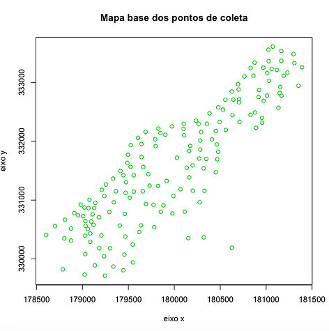
Mapa Base dos pontos de coleta
data(meuse.all)
plot(meuse.all[,2],meuse.all[,3],xlab='eixo x',ylab='eixo y',main='Mapa base dos pontos de coleta')
points(meuse.all[,2],meuse.all[,3], col=green)
-
Histograma
data(meuse.all)
g <- meuse.all
x.norm<- g$lead
h<-hist(x.norm,breaks=8)
xhist<-c(min(h$breaks),h$breaks)
yhist<-c(0,h$density,0)
xfit<-seq(0, 700, by=10)
yfit<-dnorm(xfit,mean=mean(x.norm),sd=sd(x.norm))
plot(xhist,yhist,type="s",ylim=c(0,max(yhist,yfit)),xlab="Pb",ylab="Frequência Relativa",main="Histograma de Pb ")
lines(xfit,yfit,col="green")

-
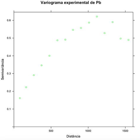
Variograma experimental
data(meuse.all)
g=gstat(id='lead',formula=log(lead)~1,locations=~x+y,data=meuse.all)
grafico=variogram(g)
plot(grafico,main=' Variograma experimental de Pb',xlab='Distância',ylab='Semivariância', col="green")
-
Variograma ajustado
data(meuse.all)
vgm1<-variogram(log(lead)~1, locations=~x+y, data=meuse.all)
x=range(vgm1[,2])
y=range(vgm1[,3])
plot(x,y, asp = 1000, type = "n", main="Variograma Ajustado")
points(vgm1[,2],vgm1[,3],col="green",cex=1.5)
lines(vgm1[,2],vgm1[,3],col="green")
f<-fit.variogram(vgm1,vgm(0.16, "Exp", 1500, 0.5))
v<-vgm(f$psill[2], "Exp",f$range[2],f$psill[1])
ff<-variogramLine(v,maxdist=1543 ,n = 15 , min = 80)
points(ff[,1],ff[,2],col = "red")
lines(ff[,1],ff[,2], col = "red")
asp=max(x)max(y)
asp=1542.27/0.6211689=2482.851

-
Box-plot
> > data(meuse.all)
m<-meuse.all
summary(m$lead)
boxplot(m$lead,horizontal=TRUE, col="green", main="Boxplot Meuse atributo Chumbo")

-
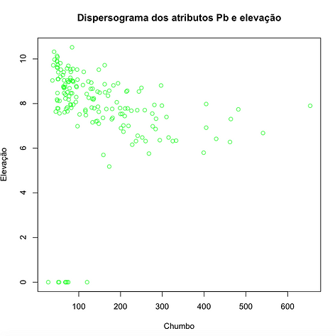
Dispersograma das variáveis
data(meuse.all)
g=gstat(id='lead')
h<-c(meuse.all)
plot(h$lead,h$elev,xlab="Chumbo",ylab="Elevação",main="Dispersograma dos atributos Pb e elevação", col="green")
-
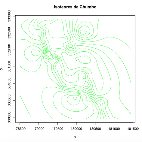
Mapa de Istoreores
s.grid<-GridTopology(c( 178500, 329965),c(60,60),c(50,50))
s.grid<-SpatialPoints(s.grid)
#spatial points
data(meuse.all)
m <- vgm(0.5643942, "Exp", 535.8096, 0.07655493)
xx <- krige(log(lead)~1, ~x+y, model = m, data = meuse.all, newd = s.grid)
dfxx<-as.data.frame(xx)
mz<-matrix(dfxx[,3], nrow=50, ncol=50, byrow=FALSE)
X11()
contour(x =seq(178500,181440,by= 60), y=seq(329965,332905,by=60),mz,nlevels=10,
xlab="x",ylab="y",main="Isoteores de Chumbo", col="green")
-
Mapa de Istoreores
s.grid<-GridTopology(c( 178500, 329965),c(60,60),c(50,50))
s.grid<-SpatialPoints(s.grid)
#spatial points
data(meuse.all)
m <- vgm(0.5643942, "Exp", 535.8096, 0.07655493)
xx <- krige(log(lead)~1, ~x+y, model = m, data = meuse.all, newd = s.grid)
dfxx<-as.data.frame(xx)
mz<-matrix(dfxx[,3], nrow=50, ncol=50, byrow=FALSE)
X11()
contour(x =seq(178500,181440,by= 60), y=seq(329965,332905,by=60),mz,nlevels=10,
xlab="x",ylab="y",main="Isoteores de Chumbo", col="green")
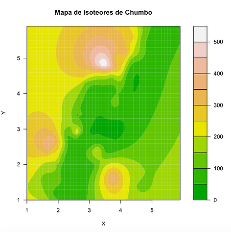
Mapa com os contornos de isoteores preenchidos:
s.grid<-GridTopology(c(178500, 329965),c(60,60),c(50,50))
s.grid <- SpatialPoints(s.grid)
data(meuse.all)
m <- vgm(0.5643942, "Exp", 535.8096, 0.07655493)
xx <- krige(lead~1, ~x+y, model = m, data = meuse.all, newd = s.grid)
dfxx <- as.data.frame(xx)
mz <- matrix(dfxx[,3], nrow=50, ncol=50, byrow=FALSE)
nmz <- matrix(nrow=50, ncol=50)
for (i in 1:50)
for (j in 1:50)
{nmz[i,j]=mz[i,51-j]}
x =seq(1.0,5.9,by= 0.1)
y=seq(1,5.9,by=0.1)
filled.contour(x, y,nmz,nlevels=10,color=terrain.colors, xlab="X",ylab="Y",main="Mapa de Isoteores de Chumbo")

-
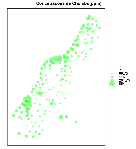
Mapa de concentração de Chumbo
data(meuse.all)
class(meuse.all)
coordinates(meuse.all)=~x+y
bubble(meuse.all, "lead", col=c("#00ff088","#00ff0088"),main="Concetrações de Chumbo(ppm)")
-
Predição do atributo baseado em krigagem ordinária
data(meuse)
coordinates(meuse)=~x+y
data(meuse.grid)
gridded(meuse.grid)=~x+y
m<- vgm(0.5232381,"Sph",880.8683, 0.1229456 )
x<-krige(log(lead)~1, meuse, meuse.grid, model = m)
spplot(x["var1.pred"], main = "Predição do chumbo em krigagem ordinária",col.regions=terrain.colors)
-
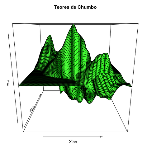
Diagrama de bloco do atributo baseado em krigagem ordinária
s.grid<-GridTopology(c(178260,329220),c(40,40),c(90,120))
s.grid<-SpatialPoints(s.grid)
#spatial points
data(meuse.all)
m<-vgm(0.5232381,"Sph",880.8683, 0.1229456)
xx<-krige(log(lead)~1,~x+y,model=m,data=meuse.all,newd=s.grid)
dfxx<-as.data.frame(xx)
mz<-matrix(dfxx[,3],nrow=90,ncol=120,byrow=FALSE)
persp(x=seq(178300,181860,by=40),y=seq(329500,334260,by=40),mz,xlab="Xloc",ylab="Yloc",main="Teores de Chumbo",col="green")
-
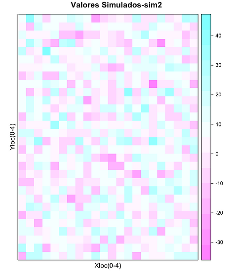
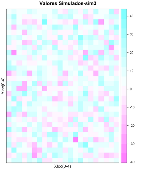
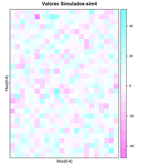
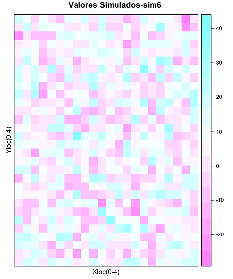
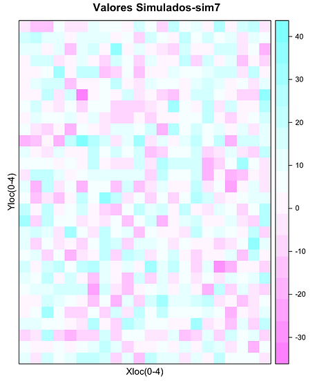
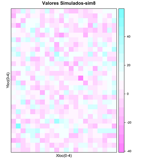
Dez simulações Gaussianas do teor de Zn expresso por cor em função localização
s.grid<-GridTopology(c(178260,329460),c(160,160),c(22.5,30))
s.grid<-SpatialPoints(s.grid)
gridded(s.grid)<-TRUE
data(meuse.all)
m<- vgm(0.56439420,"Sph",535.8096, 0. 07655493 )
xx <- krige(log(lead)~1, ~x+y, model = m, data = meuse.all, newd = s.grid )
X11()
xx <- krige(log(lead)~1, ~x+y, model = m, data = meuse.all, newd = s.grid, nsim=10)
spplot(xx["sim1"],xlab="Xloc(0-4)",ylab="Yloc(0-4)",main="Valores Simulados-sim1")
X11()
spplot(xx["sim2"],xlab="Xloc(0-4)",ylab="Yloc(0-4)",main="Valores Simulados-sim2")
X11()
spplot(xx["sim3"],xlab="Xloc(0-4)",ylab="Yloc(0-4)",main="Valores Simulados-sim3")
X11()
spplot(xx["sim4"],xlab="Xloc(0-4)",ylab="Yloc(0-4)",main="Valores Simulados-sim4")
X11()
spplot(xx["sim5"],xlab="Xloc(0-4)",ylab="Yloc(0-4)",main="Valores Simulados-sim5")
X11()
spplot(xx["sim6"],xlab="Xloc(0-4)",ylab="Yloc(0-4)",main="Valores Simulados-sim6")
X11()
spplot(xx["sim7"],xlab="Xloc(0-4)",ylab="Yloc(0-4)",main="Valores Simulados-sim7")
X11()
spplot(xx["sim8"],xlab="Xloc(0-4)",ylab="Yloc(0-4)",main="Valores Simulados-sim8")
X11()
spplot(xx["sim9"],xlab="Xloc(0-4)",ylab="Yloc(0-4)",main="Valores Simulados-sim9")
X11()
spplot(xx["sim10"],xlab="Xloc(0-4)",ylab="Yloc(0-4)",main="Valores Simulados-sim10")
X11()


-
Mapa de concentração da mediana do atributo simulado (chumbo)
s.grid<-GridTopology(c(178260,329460),c(160,160),c(30,30))
s.grid<-SpatialPoints(s.grid)
gridded(s.grid)<-TRUE
data(meuse.all)
#set.seed(9999)
m<- vgm(0.56439420,"Sph",535.8096, 0. 07655493 )
xx <- krige(log(lead)~1, ~x+y, model = m, data = meuse.all, newd = s.grid, nsim=30)
X11()
aux=matrix(1:27000,900,30)
for (i in 1:900)
for (j in 1:30)
{ aux[i,j]=xx[[j]][i]}
for (i in 1:900)
{xx[[1]][i]=median(aux[i,])}
spplot(xx[,1], xlab="xloc(0-4)", ylab="yloc(0-4)", main="Mediana")

-
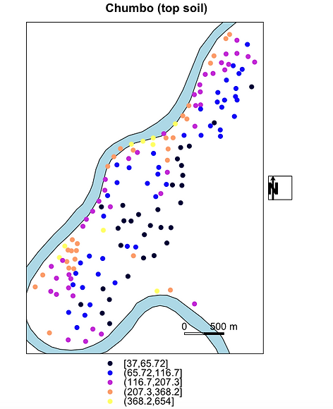
Comparação entre o Mapa de concentração da mediana do atributo simulado e o Mapa de base, com meandro do rio Meuse acrescido.
library(sp)
library(lattice) # required for trellis.par.set():
trellis.par.set(sp.theme()) # sets color ramp to bpy.colors()
data(meuse)
coordinates(meuse)=~x+y
data(meuse.riv)
meuse.sr = SpatialPolygons(list(Polygons(list(Polygon(meuse.riv)),"meuse.riv")))
rv = list("sp.polygons", meuse.sr, fill = "lightblue")
scale = list("SpatialPolygonsRescale", layout.scale.bar(),
offset = c(180500,329800), scale = 500, fill=c("transparent","black"), which = 1)
text1 = list("sp.text", c(180500,329900), "0", which = 1)
text2 = list("sp.text", c(181000,329900), "500 m", which = 1)
arrow = list("SpatialPolygonsRescale", layout.north.arrow(),
offset = c(178750,332500), scale = 400)
## plot with north arrow and text outside panels
## (scale can, as of yet, not be plotted outside panels)
spplot(meuse["lead"], do.log = TRUE,
key.space = "bottom",
sp.layout = list(rv, scale, text1, text2),
main = "Chumbo (top soil)",
legend = list(right = list(fun = mapLegendGrob(layout.north.arrow()))))